Case Study Description: To predict the trip duration of a New York taxi cab ride, we can build different types of features and evaluate them. We will start by describing what is a feature in this context; then we will develop some elementary features and add features using the software package featuretools. We will assess how these features perform in predicting trip duration.

1. Setup

Note: This uses an alternative to python’s featuretools for R called featuretoolsR

To Install featuretoolsR tou need to have “devtools” installed.
Then you can run: install_github(“magnusfurugard/featuretoolsR”)

# You wil need to define (if not already) your Python path.
# reticulate::py_discover_config()
library("reticulate")
use_python("~/Library/r-miniconda/envs/r-reticulate/bin/python")

library("featuretoolsR")
library("dplyr")
library("gbm")

1.1 Functions

featuretoolsR does not include the original encode_features python function, so a custom one was made called custom_encode_features which returns one-hot encoding of categorical variables.
Additionally, custom function to replace python SimpleImputer class and Rscores were made.

# R^2 Calculation
r_squared <- function(predicted,actual) {
  r_squared <- 1 - (sum((actual - predicted)^2) / sum((actual - mean(actual))^2))
  return(r_squared)
}

# Custom encode feature to support missing function un featuretoolsR
  custom_encode_features <- function(feature_matrix, to_encode, include_unknown, top_n) {
    temp <- feature_matrix
    for(feature in to_encode) {
      
      # We generate the list of top_n unique values for feature to encode
      if(include_unknown == TRUE) {
        encoded_feature <- names(head(sort(table(feature_matrix[[feature]],exclude = NULL),decreasing=TRUE),top_n))
      } else {
        encoded_feature <- names(head(sort(table(feature_matrix[[feature]]),decreasing=TRUE),top_n))
      }
      
      for(i in 1:length(encoded_feature)) {
        temp <- temp %>%	
          mutate( 
            !!paste(feature,"=",encoded_feature[i]) := ifelse(feature_matrix[[feature]] == encoded_feature[i] , 1, 0)
          )
      }
    }
    return(temp[,!names(temp) %in% to_encode])
  }

# Compute features function based on dsx-cs6 utils
  compute_features <- function(features,entities) {
    
    # We create feature matrix using featuretools calculate_feature_matrix function
    feature_matrix <- calculate_feature_matrix(entities,features,
                                               approximate='36d',
                                               verbose=TRUE) 
    
    # Since encode_features function is missing, we hot-encode pickup_neighborhood and dropoff_neighborhood 
    # with a custom function created: custom_encode_features
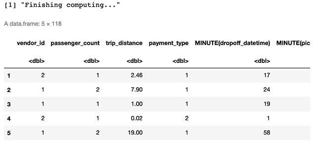
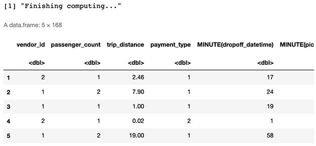
    print("Finishing computing...")
    feature_matrix <- custom_encode_features(feature_matrix, to_encode=c("pickup_neighborhood","dropoff_neighborhood"), include_unknown=FALSE, top_n=1000) 
  
    # Return Output
    return(feature_matrix)
  
  }
  
# Logical to integer
logical_to_integer <- function(feature_matrix) {
  # Convert logical values to integers
  logical_features <- names(feature_matrix[,unlist(lapply(feature_matrix, is.logical))])
  for(feature in logical_features) {
    feature_matrix[[feature]] <- as.numeric(as.integer(feature_matrix[[feature]]))
  }
  return(feature_matrix)
}

logical_to_factor <- function(feature_matrix) {
  # Convert logical values to integers
  logical_features <- names(feature_matrix[,unlist(lapply(feature_matrix, is.logical))])
  for(feature in logical_features) {
    feature_matrix[[feature]] <- as.factor(feature_matrix[[feature]])
  }
  return(feature_matrix)
}

custom_fit <- function(data) {
  out <- list()
  numeric_features <- names(data[,unlist(lapply(data, is.numeric))])
  for(feature in numeric_features) {
    out[[feature]] <- mean(data[[feature]] ,na.rm = TRUE)
  }
  return(out)
}

# Custom fit_transform
custom_transform <- function(data,fit) {
  numeric_features <- names(fit)
  for(feature in numeric_features) {
    data[[feature]][which(is.na(data[[feature]]))] <-fit[[feature]]
  }
  return(data)
}
  
# get_train_test_fm based on dsx-cs6 utils
get_train_test_fm <- function(feature_matrix, original_data, percentage) {
  
  out <- list()
  
  nrows <- nrow(feature_matrix)
  head <- nrows * percentage
  tail <- nrows - head
  
  X_train <- head(feature_matrix,head)
  y_train <- head(original_data$trip_duration,head)
  
  # Emulating fit_transform
  fit <- custom_fit(X_train)
  X_train = custom_transform(X_train,fit)
  
  X_test = tail(feature_matrix,tail)
  y_test = tail(original_data$trip_duration,tail)
  X_test = custom_transform(X_test,fit)
  
  # Return values
  out$X_train <- X_train 
  out$y_train <- y_train
  out$X_test <- X_test
  out$y_test <- y_test
  
  return(out)
  
}

1.2 Data Load

# Needed to load picke file
source_python("read_pickle.py")

Opening a pickle file in R additional info

# We load data
trips <- read_pickle_file("./trips.pkl")
dropoff_neighborhoods <- read.csv("./dropoff_neighborhoods.csv")
pickup_neighborhoods <- read.csv("./pickup_neighborhoods.csv")

# We set type
trips$pickup_neighborhood <- as.character(trips$pickup_neighborhood)
trips$dropoff_neighborhood <- as.character(as.character(trips$dropoff_neighborhood))
dropoff_neighborhoods$neighborhood_id <- as.character(dropoff_neighborhoods$neighborhood_id)
pickup_neighborhoods$neighborhood_id <- as.character(pickup_neighborhoods$neighborhood_id)

# Histogram
hist(trips$trip_duration, main="Trip Duration Distribution", 
  xlab="Trip Duration in Seconds",
  ylab="Number of Trips",
  col="lightblue")

# Tells us how many trips are in the dataset
paste("Trips in dataset:",nrow(trips))

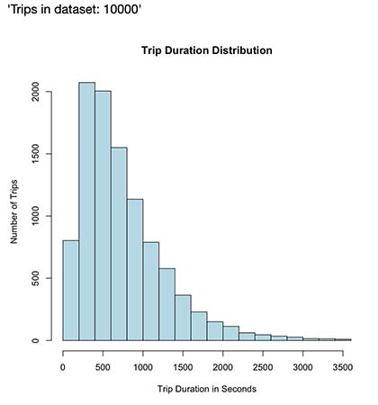
As seen in the output above, we can observe there’s 10.000 trips in the dataset. Aditionally, our histogram seems right-skewed with median around 616 seconds (10.26 minutes) and mean around 746 seconds (12.43 minutes).

1.2 Entities and Relationships

# Create entityset
entities <- as_entityset(
  trips, 
  index = "id", 
  entity_id = "trips", 
  id = "trips", 
  time_index = "pickup_datetime"
) %>%
add_entity(
  pickup_neighborhoods, 
  entity_id = "pickup_neighborhoods", 
  index = "neighborhood_id"
) %>%
add_entity(
  dropoff_neighborhoods, 
  entity_id = "dropoff_neighborhoods", 
  index = "neighborhood_id"
)

# Add index relationships
entities <- entities %>%
add_relationship(
  parent_set = "pickup_neighborhoods", 
  child_set = "trips", 
  parent_idx = "neighborhood_id", 
  child_idx = "pickup_neighborhood"
)  %>%
  add_relationship(
    parent_set = "dropoff_neighborhoods", 
    child_set = "trips", 
    parent_idx = "neighborhood_id", 
    child_idx = "dropoff_neighborhood"
  ) 

2. First Model

2.1 Transform Primitives

trans_primitives <- c("is_weekend")
features <- dfs(
  entityset=entities,
  target_entity="trips",
  trans_primitives=trans_primitives,
  agg_primitives=NULL,
  ignore_variables= list(trips=c("pickup_latitude", "pickup_longitude",
                                 "dropoff_latitude", "dropoff_longitude", "trip_duration")),
  features_only=TRUE
)
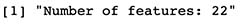
print(paste("Number of features:",length(features)))

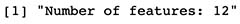
Even though some features were not included, there’s some new tranformed/generated ones:

Pickup neighborhood was transformed (hot encoded) from a categorical variable into many binary features, one for each neighborhood.
A completely new transformed feature containing whether the trip was made on a weekend was generated.

With the addition of these features we expect an increased model performance, especially due to the new engineered IS_WEEKEND feature, since both traffic flow and travel behaviors typically change between working days and weekends, therefore, these newly added features would most likely influece trip_duration, reflecting in better prediction.

2.2 Dataset Creation

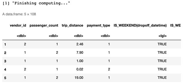
feature_matrix <- compute_features(features, entities)
head(feature_matrix,5)

2.3 Split Dataset

train_test = get_train_test_fm(feature_matrix, trips, .75)

y_train = log(train_test$y_train + 1)
y_test = log(train_test$y_test + 1)
X_train <- logical_to_integer(train_test$X_train)
X_test <- logical_to_integer(train_test$X_test)

trainingDataset = cbind(y_train,X_train)
print('Data split successful!')

2.4 Fitting Generalized Boosted Regression Model

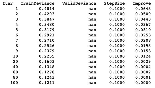
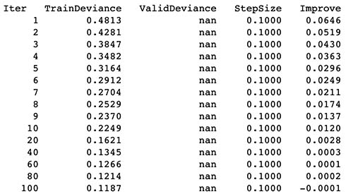
gbm <- gbm(y_train  ~ ., data = trainingDataset,verbose = TRUE,
           n.trees = 100,
           distribution="gaussian",
           interaction.depth = 3,
           n.minobsinnode = 1,
           shrinkage = 0.1)

2.5 Results from predictions

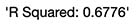
R^2

predicted_gbm <- predict(gbm,X_test,n.trees = 100)
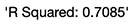
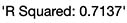
paste("R Squared:",round(r_squared(y_test,predicted_gbm),4))

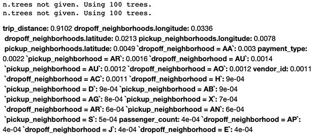
2.6 Feature Influence

head(round(relative.influence(gbm,sort= TRUE)/sum(relative.influence(gbm)),4),25)

3. Second Model

3.1 Transform Primitives

trans_primitives <- c("minute","day","week","month","weekday","is_weekend")
features <- dfs(
  entityset=entities,
  target_entity="trips",
  trans_primitives=trans_primitives,
  agg_primitives=NULL,
  ignore_variables= list(trips=c("pickup_latitude", "pickup_longitude",
                                 "dropoff_latitude", "dropoff_longitude", "trip_duration")),
  features_only=TRUE
)
print(paste("Number of features:",length(features)))

3.2 Dataset Creation

feature_matrix <- compute_features(features, entities)
head(feature_matrix,5)

3.3 Split Dataset

train_test = get_train_test_fm(feature_matrix, trips, .75)

y_train = log(train_test$y_train + 1)
y_test = log(train_test$y_test + 1)
X_train <- logical_to_integer(train_test$X_train)
X_test <- logical_to_integer(train_test$X_test)

trainingDataset = cbind(y_train,X_train)
print('Data split successful!')

3.4 Fitting Generalized Boosted Regression Model

gbm <- gbm(y_train  ~ ., data = trainingDataset,verbose = TRUE,
           n.trees = 100,
           distribution="gaussian",
           interaction.depth = 3,
           n.minobsinnode = 1,
           shrinkage = 0.1)

3.5 Results from predictions

R^2

predicted_gbm <- predict(gbm,X_test,n.trees = 100)
paste("R Squared:",round(r_squared(y_test,predicted_gbm),4))

New transform features (Minute, Hour, Day, Week, Month, Weekday) were generated in addition to Weekend Feature from the previous model. These transform features seemed to increase model performance since R^2 increased from 0.755 to 0.80.
There was very little sacrifice in terms of training time (5 secs).

3.6 Feature Influence

head(round(relative.influence(gbm,sort= TRUE)/sum(relative.influence(gbm)),4),25)

4. Third Model

4.1 Transform Primitives

trans_primitives <- c("minute","day","week","month","weekday","is_weekend")
aggregation_primitives = c("count","sum","mean","median","std","max","min")
features <- dfs(
  entityset=entities,
  target_entity="trips",
  trans_primitives=trans_primitives,
  agg_primitives=aggregation_primitives,
  ignore_variables= list(trips=c("pickup_latitude", "pickup_longitude",
                                 "dropoff_latitude", "dropoff_longitude", "trip_duration")),
  features_only=TRUE
)
print(paste("Number of features:",length(features)))

4.2 Dataset Creation

feature_matrix <- compute_features(features, entities)
head(feature_matrix,5)

4.3 Split Dataset

train_test = get_train_test_fm(feature_matrix, trips, .75)

y_train = log(train_test$y_train + 1)
y_test = log(train_test$y_test + 1)
X_train <- logical_to_integer(train_test$X_train)
X_test <- logical_to_integer(train_test$X_test)

trainingDataset = cbind(y_train,X_train)
print('Data split successful!')

4.4 Fitting Generalized Boosted Regression Model

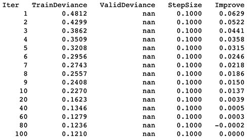
gbm <- gbm(y_train  ~ ., data = trainingDataset,verbose = TRUE,
           n.trees = 100,
           distribution="gaussian",
           interaction.depth = 3,
           n.minobsinnode = 1,
           shrinkage = 0.1)

4.5 Results from predictions

R^2

predicted_gbm <- predict(gbm,X_test,n.trees = 100)
paste("R Squared:",round(r_squared(y_test,predicted_gbm),4))

4.6 Feature Influence

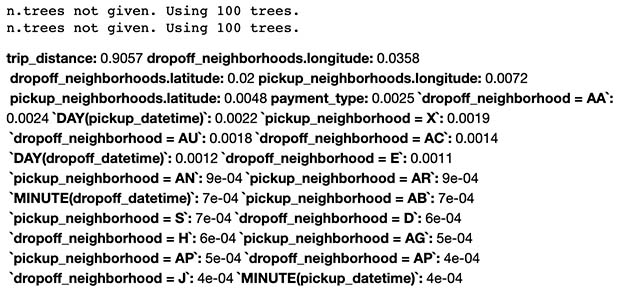
head(round(relative.influence(gbm,sort= TRUE)/sum(relative.influence(gbm)),4),25)

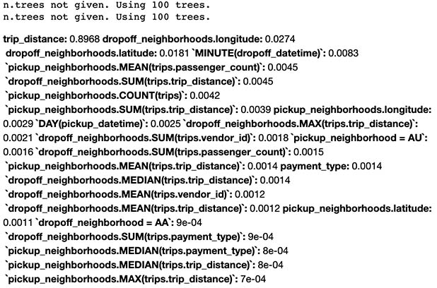
It’s coherent to see that trip_discance, pickup/drop off hour and drop off latitude/longitude would be amongst the features that most influence trip_duration, since they reflect the effect of distance, highest traffic hours and location-wise variables that would influence the trip in terms of duration.

5. Evaluation & Final thoughts

y_pred <- predict(gbm,X_test,n.trees = 100)
y_pred <- exp(y_pred) - 1 # undo the log we took earlier

y_test <- train_test$y_test

print('y_pred and y_test computation successful!')

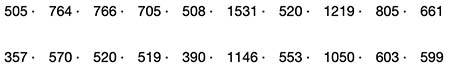
# Print the first 5 predictions and real values
head(round(y_pred),10)
head(round(y_test),10)

# Histogram of y_test
hist(y_test, main="Real Trip Duration Distribution", 
  xlab="Trip Duration in Seconds",
  ylab="Number of Trips",
  col="lightblue")
summary(y_test)

# Histogram of y_pred
hist(y_pred, main="Predicted Trip Duration Distribution", 
  xlab="Trip Duration in Seconds",
  ylab="Number of Trips",
  col="lightgreen")
summary(y_pred)

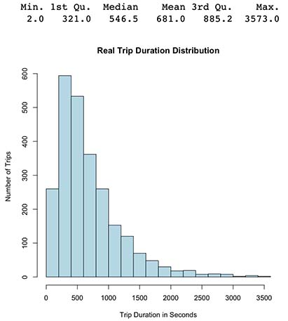
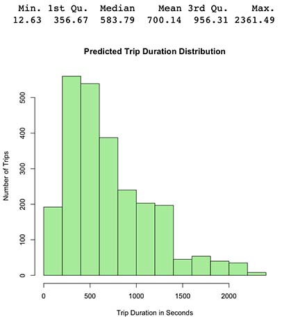
Green output histogram from our new latest model seems coherent since it’s somewhat similar to the original histogram in blue.
We can observe our prediction distribution seems to be positive/right skewed with mean 724 (original 746) and Median 594 (original 616), therefore model predictions roughly follows the same distribution as the original.
New aggregated features seems to very slightly increase model R^2, since it increased from 0.677 to 0.713 with only a minimal sacrifice of training time (+1 sec).

If more time is provided, it would be ideal to see if there’s different stacked features or depths we could explore. Additionally, domain specific knowledge could be added to generate new features or to expand information to construct with.